Introduction

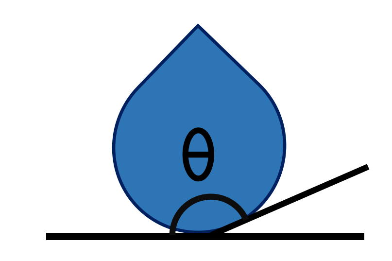
wetting_angle_kit is a Python package that analyses droplet contact angles from molecular dynamics simulations. It exposes a modular workflow: parse trajectories, recover the liquid–vapor interface, locate the wall plane, fit a geometric shape, and visualise the result.

Package Overview

The package operates in three stages: Parsing, Analysis, and Visualisation.

        graph LR
   A[Trajectory Parser] --> B[Contact Angle Analysis]
   B --> C[Visualisation]

   subgraph Parsing
   A
   end

   subgraph Methods
   B
   end

   subgraph Output
   C
   end
    

1. Trajectory Parser

The first step is to import the simulation trajectory. wetting_angle_kit supports common formats used in molecular dynamics:

	LAMMPS: .lammpstrj files are parsed natively, handling periodic boundaries and extracting specific atom types (e.g. liquid vs. wall).
	ASE: support for the Atomic Simulation Environment allows reading a wide range of trajectory formats beyond LAMMPS, plus plain .xyz files.

Each format has a paired *WaterFinder that identifies water-oxygen atoms via O–H connectivity, and an optional *WallParser for reading the wall atoms when the analysis pipeline needs them.

2. Contact Angle Analysis

The analysis layer is built around four orthogonal strategy components, each replaceable:

• Interface extractor — turns the noisy liquid atom cloud into a clean set of interface points (the liquid–vapor surface). Either a ray fan with a 1D tanh fit along each ray, or a 2D/3D density grid with an iso-density contour at the half-bulk level.

• Wall detector — locates the wall plane z-coordinate. Either derived from the interface itself (min_plus_offset), set explicitly, or read from the wall atom positions (from_atoms).

• Surface fitter — fits a geometric shape (circle per slice, or a single sphere/cylinder) to the interface points and reports the cap/wall intersection angle.

• Temporal aggregator — groups frames into batches: per-frame, pooled by N, or fully pooled.

Two top-level entry points compose these strategies in different ways.

Top-level analyzers

TrajectoryAnalyzer is the composable pipeline: you pick an extractor, a wall detector, a surface fitter, and a temporal aggregator, and the analyzer runs them per batch. Examples of useful combinations:

• ray-fan sampling + slicing fit + min_plus_offset wall + per-frame batches — a per-frame angle trace with a per-slice ±σ band;

• ray-fan sampling + whole-fit + explicit wall + 10-frame pooled batches — a whole-shape sphere fit with the wall position imported from the simulation setup;

• grid sampling + slicing fit + from_atoms wall + per-frame batches — interface from a 2D density iso-contour, wall from the actual substrate atoms.

CoupledFit2DAnalyzer and CoupledFit3DAnalyzer are the coupled-fit alternative. They skip the extractor/wall/fitter decomposition and fit a seven-parameter (2D) or nine-parameter (3D) hyperbolic-tangent density model directly to the binned density. One robust angle per batch; ideal when you have many frames per batch and don’t need per-frame time resolution.

Supported geometries

All methods can analyse:

• spherical droplets — standard spherical-cap shapes,

• cylindrical droplets — cylindrical droplets along the x or y axis (e.g. water on a nanowire or a periodic stripe).

Note

Both methods recenter the droplet per frame using a periodic-image-aware (circular-mean) construction. Trajectories where the droplet drifts during the run, or where atoms wrap across a periodic boundary, are handled transparently. Producing a pre-recentered trajectory at simulation time is optional, though still convenient for visualisation and post-processing:

fix recenter group_id INIT INIT NULL

All methods require the simulation box to be large enough so that the droplet does not interact with its periodic image (i.e. its lateral diameter is comfortably below the box length). If that condition is violated, the radial density profile is physically meaningless regardless of the centering strategy.

3. Visualisation

Three visualisation classes cover the most common needs:

• AngleEvolutionPlotter — per-batch contact angle vs time, with an optional ±σ band (per-slice scatter for the slicing fitter, bootstrap σ for the whole fitter) and a cumulative running mean overlay.

• DensityContourPlotter — 2D density field with the fitted spherical cap and wall line overlaid; accepts a single batch or a full results object (averaged density), and also collapses 3D results azimuthally onto the same plot.

• DropletSlicePlotter — single-frame snapshot of the droplet with the fitted circle, surface contour, and tangent at the contact point.

Examples for each plot live in the Tutorials section.

4. Parallelisation and progress reporting

Every analyzer (TrajectoryAnalyzer, CoupledFit2DAnalyzer, CoupledFit3DAnalyzer) accepts an n_jobs argument on analyze() for worker-process parallelism, plus a temporal_aggregator constructor argument that controls how the requested frame range is partitioned into batches. The two interact in three regimes:

• Per-frame analysis (batch_size=1, the default for TrajectoryAnalyzer): each frame is its own batch, so n_jobs > 1 distributes batches over a multiprocessing.Pool. This is the right combination for long trajectories where you want a time-resolved angle trace and CPU cores are the limiting resource.

• Bucketed batches (batch_size=N, N > 1): consecutive groups of N frames are pooled into batches; n_jobs > 1 distributes those batches across workers. Each batch gives one pooled-density fit and angle_std reports spatial asymmetry of the pooled cloud (see the note on pooled-batch slicing in the Tutorial: Contact Angle Analysis (Slicing Pipeline)).

• Fully pooled (batch_size=-1, the default for the coupled-fit analyzers): every frame goes into one batch and one fit. Because there’s only one unit of work, n_jobs is silently irrelevant — analyze() always runs inline, and passing n_jobs > 1 emits a UserWarning to flag the wasted expectation. Reach for batch_size=-1 when you want one maximally-noise-reduced angle over a steady-state window.

The multiprocessing.Pool uses the spawn start method, so trajectory parsers are reconstructed in each worker from the file path captured at TrajectoryAnalyzer.__init__. Keep parser construction cheap (just a path string and a few light flags) — the spawn cost shows up once per worker per analyze() call.

Progress is reported in frames, not batches, so the tqdm meter stays informative regardless of batch_size. Under batch_size=-1 the meter still updates frame-by-frame while the per-frame parse loop runs at the start of the batch; the subsequent extract/fit stage on the pooled cloud is opaque to the meter (a single long-running computation that the workers can’t subdivide).

Troubleshooting

• NaN angles: usually mean the surface filter removed too many points (empty slice). Raise the offset on SurfaceFitter.slicing() (surface_filter_offset) or relax the slicing step. Make sure each slice has ≥3 surviving interface points for the circle fit.

• Misconfiguration errors at construction: TrajectoryAnalyzer validates the extractor / fitter / wall detector trio in __init__ — a ValueError at construction catches incompatible configurations before any trajectory I/O happens. Read the message: it names the constraint that was violated.

• Multiprocessing hangs: the batched analyzers use the spawn start method. Avoid invoking OVITO parsers at module top level before multiprocessing starts; pass file paths instead and let each worker rebuild its own parser.

• OVITO ImportError: install with the ovito extra or via the Conda command listed in the installation section. Verify channel priority and version pin if dependency resolution fails.

• Whole-fit angle off by tens of degrees: pair the whole fitter with WallDetector.explicit() or WallDetector.from_atoms() rather than WallDetector.min_plus_offset() when the difference between the interface-derived baseline and the physical wall is large enough to matter for your droplet’s geometry.