Tutorial: Contact Angle Analysis (Slicing Pipeline)

This tutorial walks through the slicing pipeline built from the strategy components of TrajectoryAnalyzer: a ray-fan interface extractor, a per-slice algebraic-circle fitter, and an interface-derived wall detector. The slicing pipeline is the right choice when you want a per-frame angle trace plus a sense of the spread across slices.

1. How it works 

The pipeline does three things per batch:

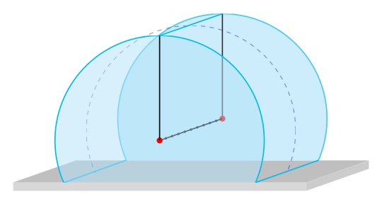
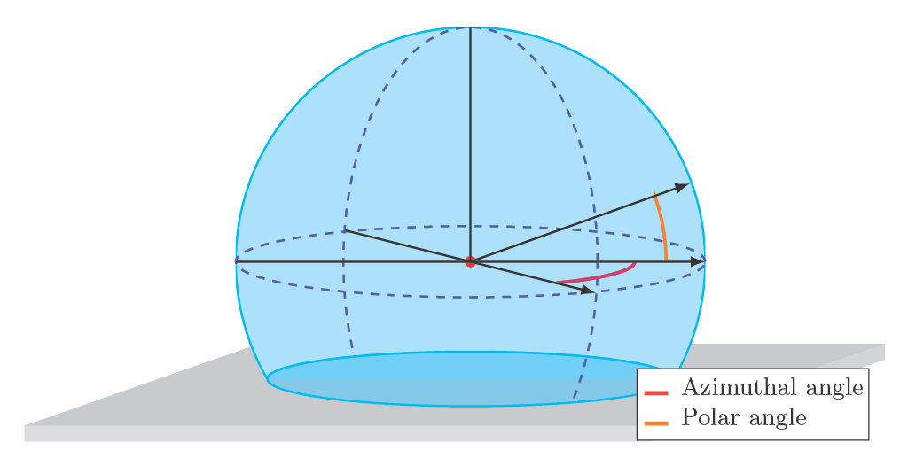
Interface extraction. The droplet is divided into vertical slicing planes (azimuthal slices for a spherical droplet, y-step slices for a cylindrical droplet). Inside each plane a 2D ray fan emits rays from the droplet centre of mass and locates the interface along each ray as the half-density point of a 1D tanh fit on the local density profile (Gaussian KDE by default).
Wall detection. The wall plane z-coordinate is taken as the minimum z over all interface points, plus a user-supplied offset (min_plus_offset(offset=0) for the bare baseline).
Surface fit. An algebraic Taubin circle is fit to each slice’s interface points after filtering out points within surface_filter_offset of the wall. The contact angle on each slice is the angle of intersection of that circle with the wall line; the batch’s reported angle is the mean across slices, and SlicingBatchResult.angle_std is the empirical std.

1.1 Ray parameter quick-reference 

When configuring SpaceSampling.rays(), the required parameters depend on which (surface_kind, droplet_geometry) pair the sampling is paired with. The table below summarises the mapping:

surface_kind	geometry	required ray params
slicing	spherical	`delta_azimuthal` (+ `delta_polar`)
slicing	cylinder_x / cylinder_y	`delta_cylinder` (+ `delta_polar`)
whole	spherical	`n_rays_sphere`
whole	cylinder_x / cylinder_y	`delta_cylinder` (+ `delta_polar`)

../_images/wetting_angle_kit_cylinder.jpg

../_images/wetting_angle_kit_3d_droplet.png

Parameter glossary:

delta_azimuthal — azimuthal step (degrees) between slicing planes for a spherical droplet.
delta_cylinder — step (Å) along the cylinder axis between slicing planes for a cylindrical droplet (used by both slicing and whole modes).
delta_polar — in-plane ray step (degrees). Shared by every mode except whole + spherical (which uses a Fibonacci ray fan instead of per-plane polar rays). Default: 8°.
n_rays_sphere — total number of Fibonacci-distributed rays over the full sphere (whole + spherical only). Full-sphere coverage — including downward rays — is intentional: downward rays from the COM hit the wall plane and produce interface points at \(z \approx z_w\), which keeps WallDetector.min_plus_offset() consistent.

Passing parameters that don’t match the (surface_kind, geometry) pair is silently ignored; omitting a required one raises at construction time via SpaceSampling.validate_compatibility().

1.2 Key tuning knobs 

Slicing step (delta_azimuthal for spherical droplets, delta_cylinder for cylinders): smaller step → more slices, more detail per batch, more cost. The default 20° gives 9 slices for a spherical droplet, plenty for a stable mean.
In-plane ray step (delta_polar, both geometries): smaller step → more rays per slice, denser interface contour, more cost.
Wall offset (WallDetector.min_plus_offset(offset=O)):raise O if the interface-derived baseline lands slightly into the wall layer (visible as inflated angles).
Surface filter offset (SurfaceFitter.slicing(surface_filter_offset=...)): excludes interface points within this distance of the wall before the circle fit. Raise it if the wall-adjacent density is distorted by layering.

2. Minimal working example 

Before running the example, ensure you have installed the package with the ovito extra (for LAMMPS dump files):

pip install wetting-angle-kit[ovito]
# (and the OVITO package itself via conda — see installation page)

Example trajectory:

tests/trajectories/traj_spherical_drop_4k.lammpstrj

from wetting_angle_kit.analysis import (
    DensityEstimator,
    InterfaceExtractor,
    SpaceSampling,
    SurfaceFitter,
    TrajectoryAnalyzer,
    WallDetector,
)
from wetting_angle_kit.analysis.temporal import TemporalAggregator
from wetting_angle_kit.parsers import LammpsDumpParser, LammpsDumpWaterFinder

# --- Step 1: Define the trajectory file ---
filename = "../../tests/trajectories/traj_spherical_drop_4k.lammpstrj"

# --- Step 2: Identify water-oxygen atoms ---
wat_find = LammpsDumpWaterFinder(
    filename,
    oxygen_type=1,
    hydrogen_type=2,
)
oxygen_indices = wat_find.get_water_oxygen_indices(frame_index=0)
print("Number of water molecules:", len(oxygen_indices))

# --- Step 3: Build the trajectory analyzer ---
# Strategies: rays extractor (Gaussian) + slicing fitter +
# interface-derived wall + per-frame batching.
analyzer = TrajectoryAnalyzer(
    parser=LammpsDumpParser(filename),
    atom_indices=oxygen_indices,
    droplet_geometry="spherical",
    interface_extractor=InterfaceExtractor(
        sampling=SpaceSampling.rays(
            delta_azimuthal=20.0,  # 20° between slicing planes
            delta_polar=8.0,  # 8° in-plane ray step
        ),
        density=DensityEstimator.gaussian(),
    ),
    surface_fitter=SurfaceFitter.slicing(surface_filter_offset=2.0),
    wall_detector=WallDetector.min_plus_offset(offset=0.0),
    temporal_aggregator=TemporalAggregator(batch_size=1),  # one angle per frame
)

# --- Step 4: Run the analysis on a frame range ---
results = analyzer.analyze(range(0, 24))

# --- Step 5: Inspect the results ---
print("Mean contact angle (°):", results.mean_angle)
print("Std across batches (°):", results.std_angle)
for batch in results.batches[:3]:
    print(
        f"Frame {batch.frames[0]}: "
        f"angle (mean) = {batch.angle:.2f}°, "
        f"angle (median) = {batch.median_angle:.2f}°, "
        f"per-slice σ = {batch.angle_std:.2f}°, "
        f"rms residual = {batch.rms_residual:.2f} Å"
    )

3. Understanding the results 

On the water/graphene fixture above, single-frame output looks like:

Number of water molecules: 1320
Mean contact angle (°): 95.16
Std across batches (°): 0.0
Frame 0: angle (mean) = 95.16°, angle (median) = 95.02°, per-slice σ = 1.86°, rms residual = 0.45 Å

std_angle is 0 here because only one batch was requested; pass a multi-frame range to see the spread across batches.

3.1 Per-batch fields 

The returned TrajectoryResults object holds a list of SlicingBatchResult entries (one per batch). Each batch carries:

angle — mean contact angle across slices (°). This is nanmean(per_slice_angles).
median_angle — median contact angle across slices (°). More robust than the mean when one or two slices are outliers (e.g. due to asymmetric density near the periodic boundary).
angle_std — empirical standard deviation across slices (°).
per_slice_angles — full array of per-slice angles (nan for slices that produced no valid fit).
slice_surfaces / slice_popts — per-slice interface points and fitted circle parameters (for plotting; see Visualisation Tutorial — Per-Frame Droplet Snapshot).
z_wall — wall position used by the fitter.
rms_residual — mean of per-slice circle-fit RMS residuals (Å).
n_slices_total / n_slices_used — total slices vs. how many produced a valid angle. A gap signals per-slice attrition.

3.2 Mean vs. median 

Both angle (the mean) and median_angle are computed from the same per_slice_angles array, ignoring nan entries. The median is the recommended default when reporting a single number, because a single outlier slice (e.g. a nearly empty azimuthal plane near a periodic edge) can pull the mean significantly. When the distribution across slices is symmetric, mean and median agree.

The AngleEvolutionPlotter supports both via its stat parameter ("median" by default).

4. Common configurations 

4.1 Cylindrical droplets 

Use “cylinder_x” when the cylinder axis is x. Use “cylinder_y” when the cylinder axis is y Picking the wrong axis is the cylinder analogue of confusing the in-plane radial direction with the symmetry axis;could lead to NaNs angles output or non-physical angle:

4.2 Binning density estimator 

The same ray-fan geometry is available with a 1D histogram density estimator instead of the Gaussian KDE. Use it when you want a hard-cutoff per-sample density (fast, no smoothing parameter beyond the bin width):

interface_extractor = InterfaceExtractor(
    sampling=SpaceSampling.rays(
        delta_azimuthal=20.0,
        delta_polar=8.0,
        points_per_angstrom=1.0,
    ),
    density=DensityEstimator.binning(bin_width=3.0),  # 3 Å diameter top-hat
)

The bin_width parameter sets the diameter of the 3D top-hat counted at each sample point along the ray; matching it to the interface thickness (~1–3 Å for water) keeps the tanh fit well-conditioned. Numerically the bin width plays the same role density_sigma plays for rays (Gaussian).

4.3 Pooled batches 

Replace batch_size=1 with batch_size=N to pool \(N\) consecutive frames per fit — fewer batches, more atoms per fit, less per-angle noise but no within-batch time resolution. batch_size=-1 pools all requested frames into a single batch (one angle for the whole trajectory).

temporal_aggregator = TemporalAggregator(batch_size=5)

Note

With batch_size > 1, the temporal aggregator pools atom positions across frames (after per-frame PBC recentring) before the extractor runs. The slicing pipeline then operates on a single density field built from the union of frames, giving one angle per batch with angle_std reflecting the spatial asymmetry of the pooled density — not per-frame variability. This is the right tool if you want a robust single angle over a steady-state window, with the per-slice scatter as an asymmetry diagnostic.

If you want per-frame angles plus their across-frame mean and standard error, use batch_size=1 and aggregate the angles yourself from the returned per_batch_angles array. The two modes are statistically different: pooled-atoms averages the density before measuring; pooled-angles measures each frame and then averages.

Two subtle caveats of pooled-atoms mode: translational drift across the batch is handled (per-frame PBC recentring), but rotational drift and shape oscillations are smeared together with the spatial asymmetry. For steady-state droplets this is harmless; for transient regimes (wetting, dewetting, vibration) batch_size=1 is the correct choice.

4.4 Grid alternative 

The grid extractor (SpaceSampling.grid()) pairs with the slicing fitter exactly the same way and is covered in Tutorial: Grid-Based Space Sampling for Interface Extraction. Use it when ray-fan sampling is too sparse to resolve the interface.

5. Further reading 

Theoretical foundations: the physics behind each ray-fan layout and the Taubin circle fits are detailed in Theoretical foundations (§3.2 for sampling, §4 for the Taubin fit, §5 for wall detection, §8 for frame batching).
Visualization: for a side-by-side plot of the recovered interface and the fitted circle, see Visualisation Tutorial — Per-Frame Droplet Snapshot.
Angle evolution: to plot the per-batch angle trace over time (mean or median, with running-mean overlay), see Visualisation Tutorial — Angle Evolution and Density Contour.
Whole-fit pipeline: for a single-fit approach on the full 3D interface shell (with optional bootstrap uncertainty), see Tutorial: Whole-Shape Fit with Bootstrap Uncertainty.
Coupled fit: for the NLLS coupled model that fits interface + wall simultaneously, see Tutorial: Contact Angle Analysis (Coupled Fit, 2D) (2D) and Tutorial: 3D Coupled-Fit Analyzer (3D).