Theoretical foundations

This section presents the physics and numerics behind wetting_angle_kit, from the contact-angle definition to the extraction, wall detection, and fitting strategies of the analyzers.

1. The contact angle and the cap geometry

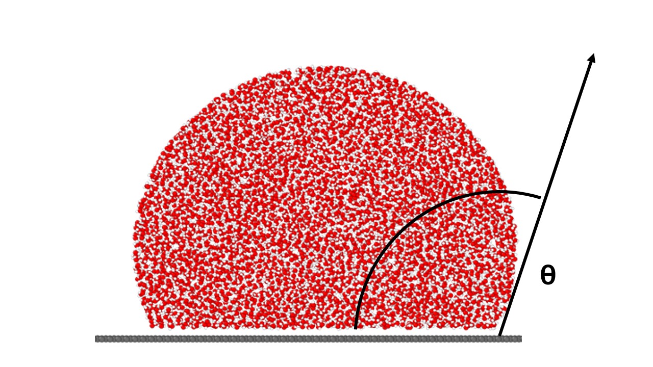
The contact angle \(\theta\) is the angle between the tangent to the liquid-vapor interface and the wall surface, measured through the liquid. For an idealised spherical-cap droplet of radius \(R\) whose centre sits at height \(z_c\) above the wall plane \(z = z_w\), simple geometry gives

\[\cos \theta \;=\; \frac{z_w - z_c}{R}.\]

Physically:

• \(z_c < z_w\) (sphere centre below the wall) ⇒ \(\cos \theta > 0\) ⇒ \(\theta < 90^\circ\): hydrophilic.

• \(z_c = z_w\): \(\theta = 90^\circ\) (hemisphere).

• \(z_c > z_w\): \(\cos \theta < 0\) ⇒ \(\theta > 90^\circ\): hydrophobic.

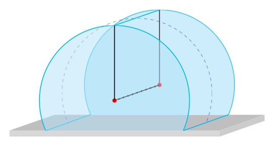
The same identity governs cylindrical droplets, replacing the spherical cap by a circular cross-section in the plane perpendicular to the cylinder axis.

The job of the analysis pipeline is to estimate \(R\), \(z_c\), and \(z_w\) from atom positions, robustly enough that the recovered \(\theta\) is meaningful.

2. Geometric symmetry classes

Three geometries are supported via DropletGeometry:

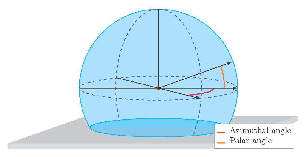
• "spherical" — full 3D droplet with no special axis.

• "cylinder_y" — cylindrical droplet along the \(y\) axis.

• "cylinder_x" — cylindrical droplet along the \(x\) axis.

The geometry choice cascades through every component:

• spherical droplets are treated as fully three-dimensional objects;

• cylindrical droplets exploit translational symmetry along the cylinder axis and can therefore be reduced to a two-dimensional fitting problem;

• the sampling strategy, wall detection, and fitting procedure are automatically adapted to the selected geometry.

The cylindrical and spherical geometries share the same fitting framework and contact-angle definition. The only difference is that the cylindrical analysis is performed on cross-sections along the cylinder axis rather than on azimuthal slices.

3. The liquid–vapor interface in MD trajectories

There is no sharp surface in an MD frame: the density drops from \(\rho_{\rm liq}\) to \(\rho_{\rm vap}\) smoothly over a few Å, broadened by thermal motion. The package treats the liquid–vapor interface as the locus of half-bulk density. This interface is then used to fit a circle/sphere and recover the contact angle. The extraction of the interface is based on two choices:

• The density field may be computed via a Gaussian KDE or a 3D top-hat binning.

• The density may be sampled along rays from the droplet Center of Mass (COM) or on a fixed grid in space.

3.1. Estimating local density

We first need a local density estimate at each sample point. Two estimators are available, swappable via DensityEstimator:

Gaussian KDE

Each atom contributes a normalised 3D Gaussian of width \(\sigma\):

\[\rho_{\rm KDE}(\mathbf{r}) \;=\; \sum_i \frac{1}{(2\pi)^{3/2}\sigma^3}\, e^{-\|\mathbf{r} - \mathbf{r}_i\|^2 / 2\sigma^2}.\]

Smooth and bias-controlled (the only knob is \(\sigma\)), which makes it the default choice. For efficiency, a per-atom cut-off at \(5\sigma\) is applied via a cKDTree.

3D top-hat

Atoms within \({\rm bin\_width}/2\) of the sample contribute uniformly:

\[\rho_{\rm bin}(\mathbf{r}) \;=\; \frac{N(\mathbf{r}, {\rm bin\_width}/2)}{V_{\rm bin}}.\]

Fast and conceptually simple, but the hard cut-off introduces Poisson noise that can interfere with the tanh fit unless the bin width is matched to the smoothing length you’d otherwise pick.

Both estimators implement the same DensityFieldProtocol, so the analysis pipeline can plug either one into the same ray-fan or grid extraction.

3.2. Sampling the density field

Two strategies turn the density estimator into a clean point set on the interface:

Ray fans

The SpaceSampling.rays() factory emits a fan of rays from the droplet COM, samples the density along each ray, and recovers the interface position as the half-density point of a 1D tanh fit on that ray.

In such samplings, the interface is recovered by fitting a one-dimensional hyperbolic-tangent profile to the density sampled along each ray:

\[\rho(\zeta) \;=\; h \;+\; d\,\tanh(\zeta_d - \zeta),\]

where \(\zeta\) is the running coordinate along the ray and the three fitted parameters are the interface location \(\zeta_d\), the midpoint density \(h = (\rho_{\rm liq} + \rho_{\rm vap})/2\), and the half-amplitude \(d = (\rho_{\rm liq} - \rho_{\rm vap})/2\). The interface is \(\zeta = \zeta_d\), where \(\rho = h\).

The transition width is fixed — the tanh argument has unit slope, giving a transition scale of order 1 Å — rather than being a fitted parameter. Because the profile is antisymmetric about its midpoint, the recovered half-density crossing \(\zeta_d\) is largely insensitive to the exact width, so fixing the slope instead of fitting a thickness does not bias the interface location; only the amplitude/width interpretation would change, and the downstream geometry never uses it. (The coupled fit of §5 does treat the interface thicknesses \(t_1, t_2\) as free parameters, because there the full density field — not just the crossing — is modelled.)

This tanh profile is theoretically motivated by mean-field theory of liquid–vapor interfaces (van der Waals / Cahn–Hilliard square-gradient free energy) and is an excellent empirical fit to MD density profiles in the same regime.

Four ray-fan geometries are used depending on the (surface_kind, droplet_geometry) pair:

• slicing + spherical: a 2D ray fan in each azimuthal plane through the droplet (planes spaced by delta_azimuthal); within each plane, rays at polar angles spaced by delta_polar.

• slicing + cylinder: a 2D ray fan in each y-step plane (planes spaced by delta_cylinder); same polar fan within each plane.

• whole + spherical: a full-sphere Fibonacci ray fan from the COM. Equal-area in \((\cos\theta, \phi)\) with the golden angle in \(\phi\); total ray count is n_rays_sphere. Full-sphere coverage is important: downward rays from the COM hit the wall plane and produce shell points at \(z \approx z_w\), which is what makes WallDetector.min_plus_offset() work for the whole-fit.

• whole + cylinder: at each step along the cylinder axis (spaced by delta_cylinder), a 2D ray fan is cast in the plane perpendicular to that axis; the full interface shell is the union of all per-step rings.

The choice of Fibonacci on the sphere is motivated by the fact that naive uniform \((\theta, \phi)\) gridding clusters rays near the poles, oversampling there and undersampling the equator. The Fibonacci spiral (uniform \(\cos\theta\), golden angle \(\phi\)) gives near-perfect equal-area coverage without clusters.

Grid + iso-contour

The SpaceSampling.grid() factory builds a fixed-cell grid in space and computes a density value at each cell, then recovers the interface as the iso-density contour at the half-bulk level via skimage.measure.find_contours() in 2D (marching squares) or skimage.measure.marching_cubes() in 3D.

In slicing mode, the grid sampling iterates per slice — azimuthal angles γ ∈ [0°, 180°) for spherical droplets, axial steps along y for cylinder droplets — exactly like the rays variant. Each slice yields an (s, z) density field and one iso-contour; the downstream SurfaceFitter.slicing averages the per-slice angles and reports the inter-slice scatter, which is how the slicing method exposes droplet asymmetry.

Two volume-normalisation notes:

• grid + gaussian returns 3D density per ų directly from the KDE evaluation; no extra volume normalisation needed.

• grid + binning’s slab-cut histogram divides by ds × dz × dx so the recovered field is also in atoms/ų. The slab thickness equals dx (the in-plane horizontal cell width), which keeps the bin’s cross-section in the (s, perpendicular) directions square.

4. Fitting the cap: algebraic Taubin fits

Given a clean point set on the interface, the surface fitter recovers the spherical-cap parameters \((z_c, R)\) (and \((x_c, y_c)\) in 3D) via an algebraic Taubin fit.

A circle/sphere is the zero set of \(g(\mathbf{r}) = A\,\|\mathbf{r}\|^2 + \mathbf{b}\cdot\mathbf{r} + c\) (a circle/sphere whenever \(A \neq 0\), with centre \(\mathbf{r}_c = -\mathbf{b}/(2A)\) and radius \(R = \sqrt{\|\mathbf{b}\|^2/(4A^2) - c/A}\)). The Taubin fit recovers the coefficients by minimising the algebraic residual normalised by its gradient,

\[\min_{A,\,\mathbf{b},\,c} \; \frac{\sum_i g(\mathbf{r}_i)^2} {\sum_i \|\nabla g(\mathbf{r}_i)\|^2}.\]

The solution is closed-form: after centring the data it is the smallest right singular vector of a small design matrix (one SVD, no iteration and no initial guess). The 2D circle fit is the same construction with the \(y\) column dropped.

The gradient normalisation largely removes the bias that algebraic fits can exhibit on incomplete arcs. This is precisely the situation encountered for droplets, where only a portion of the underlying circle is observable. Since the recovered radius feeds directly into \(\cos\theta = (z_w - z_c)/R\), accurate fitting of partial arcs is essential. On synthetic datasets, Taubin fits agree with full orthogonal-distance fits to better than \(0.1^\circ\), while remaining a closed-form method that requires neither an initial guess nor numerical iteration.

The slicing fitter (SurfaceFitter.slicing()) runs one Taubin circle fit per slice in the slice’s (x, z) plane, then averages the per-slice angles. The whole fitter (SurfaceFitter.whole()) runs one Taubin sphere fit (spherical droplet) or one Taubin circle fit (cylindrical droplet, exploiting translational symmetry along \(y\)) on the entire shell.

5. Locating the wall plane

The contact angle is read from the cap–wall intersection, so the wall plane \(z_w\) has to be located explicitly:

• WallDetector.min_plus_offset() — derive \(z_w\) from the interface itself, as \(z_w = \min(z_{\rm interface}) + \mathrm{offset}\). For slicing extractors the minimum across all slices’ interface points is taken on the contact line; for the full-sphere ray fan, downward rays from the COM reach the wall plane, so \(\min(z_{\rm shell})\) is again physically meaningful.

• WallDetector.from_atoms() — read wall-atom positions from the trajectory and place \(z_w\) at the mean of the top atomic layer (atoms within top_layer_tolerance of the highest wall atom). Physically faithful when the simulation explicitly models the substrate.

• WallDetector.explicit() — caller supplies \(z_w\) directly. Useful when the wall position is known a priori from the simulation setup (e.g. a Lennard-Jones 9-3 wall at a known \(z\)-coordinate).

A consequence worth remembering: the recovered angle is sensitive to the wall position via the cap geometry \(\cos \theta = (z_w - z_c)/R\). A 1.5 Å shift in \(z_w\) on a 25 Å droplet at \(\theta \approx 95^\circ\) corresponds to roughly a 3° shift in the recovered angle. So either pick the wall detector that matches your trust budget, or report the angle for two choices to make the dependence visible.

6. Coupled fit

The CoupledFit2DAnalyzer and CoupledFit3DAnalyzer skip the extractor/wall/fitter decomposition and fit a multi-parameter density model directly to a density field on a fixed grid.

The per-cell density is computed by the same pluggable DensityEstimator strategy used elsewhere in the package: either a top-hat histogram (DensityEstimator.binning(), the default) or a 3D Gaussian KDE evaluated at the cell centres (DensityEstimator.gaussian()). The binning variant is fast and exact but intrinsically noisy at low per-cell atom counts; the Gaussian variant smooths out Poisson noise at the cost of a small constant overhead per batch. The choice of estimator does not affect the model or the fit procedure — only the density values fed into the NLLS solver.

6.1 The 2D model (7 parameters)

After projecting atoms to (xi, zi) via the droplet symmetry, the analyzer computes a per-cell density and fits

\[\rho(\xi, z) \;=\; g(r) \cdot h(z - z_0), \qquad r = \sqrt{\xi^2 + (z - z_c)^2},\]

with

\[g(r) \;=\; \tfrac{1}{2}\bigl[(\rho_1 + \rho_2) - (\rho_1 - \rho_2)\tanh\!\bigl(2(r - R_{eq})/t_1\bigr)\bigr], \qquad h(\eta) \;=\; \tfrac{1}{2}\bigl[1 + \tanh\!\bigl(2 \eta / t_2\bigr)\bigr].\]

The radial sigmoid \(g(r)\) describes the spherical-cap interface; the vertical sigmoid \(h(z - z_0)\) cuts off the density below the wall plane \(z_0\). The seven free parameters \((\rho_1, \rho_2, R_{eq}, z_c, z_0, t_1, t_2)\) are fit simultaneously by a bounded nonlinear least-squares (scipy.optimize.curve_fit()).

The contact angle follows directly:

\[\cos \theta \;=\; \frac{z_0 - z_c}{R_{eq}}.\]

6.2 The 3D model (9 parameters)

The 3D extension computes a density on a full (xi, yi, zi) Cartesian grid and fits

\[\rho(\xi, \eta, z) \;=\; g(r) \cdot h(z - z_0), \qquad r = \sqrt{(\xi - \xi_c)^2 + (\eta - \eta_c)^2 + (z - z_c)^2},\]

with two extra parameters \(\xi_c, \eta_c\) for the horizontal centre. Nine free parameters; same cap geometry for \(\theta\). Spherical droplets only (cylindrical droplets are rejected at construction because translational symmetry along the cylinder axis already collapses the 3D problem onto the 2D one).

6.3 Why a coupled fit?

The coupled fit shares information across the cap and the wall: the radial sigmoid is constrained by the apex curvature and the contact line simultaneously, and the vertical sigmoid pins the wall plane against the cap’s lower extent. Statistically more efficient than the decoupled pipeline when you can afford to pool many frames per batch; less informative per batch (single angle) and slower per batch (a 7-parameter NLLS rather than one closed-form Taubin solve per slice).

7. Periodic boundaries and droplet recentering

MD simulations are run with periodic boundary conditions; a droplet that drifts during the run can end up “split” across an \(x\) or \(y\) periodic edge by the time you analyse a given frame. A naive arithmetic mean of the atom positions would then place the “centre” inside the empty vapor region between the two halves of the droplet, ruining every downstream computation.

wetting_angle_kit uses a circular-mean recentering that handles this automatically. For each periodic direction \(u \in \{x, y\}\), atom positions \(u_i\) are first mapped to the unit circle:

\[\phi_i \;=\; 2\pi \, u_i / L_u, \qquad \bar\phi \;=\; {\rm atan2}\!\Bigl(\textstyle\sum_i \sin\phi_i, \;\textstyle\sum_i \cos\phi_i\Bigr).\]

The mean angle \(\bar\phi\) is the circular mean; the recentered atom positions are then

\[u_i' \;=\; ((u_i - L_u\bar\phi/(2\pi) + L_u/2) \bmod L_u) - L_u/2,\]

i.e. fold every atom into the box such that the droplet is centred on the box’s middle. Trajectories where the droplet drifts or wraps across a periodic edge are handled transparently; producing a pre-recentered trajectory at simulation time is optional.

The single precondition is that the simulation box must be large enough that the droplet does not interact with its periodic image — i.e. the droplet’s lateral diameter must be comfortably below the box length. If that condition is violated, the radial density profile is physically meaningless regardless of the centering strategy.

8. Frame batching

The TemporalAggregator groups trajectory frames into batches before the full pipeline runs. Three regimes are useful:

batch_size=1

One pipeline run per frame. Best for time-resolved studies; the per-frame angle_std (per-slice scatter for slicing fits, bootstrap σ for whole fits) reports the within-frame uncertainty.

batch_size=N

Pool \(N\) consecutive frames before the fit. Fewer batches, more atoms per fit → less noise per angle, but you lose time resolution within each batch.

batch_size=-1

Pool every requested frame into a single batch — one angle for the whole trajectory. The default for the coupled-fit analyzers; useful for the slicing/whole pipeline too when you only want a representative angle.

The trade-off: the per-batch fit cost scales with the number of atoms in the batch (roughly linearly for ray fans, sub-linearly for grid binning), but the noise on the recovered angle scales inversely with \(\sqrt{N}\) in regimes where shot noise dominates. For a 4k-atom droplet on a typical room-temperature trajectory, batch_size between 1 and 10 covers the useful range.

9. Modular Workflow

The following diagram summarises the composable components of the analysis module and how they connect:

        flowchart TD
    %% ---------- role styles ----------
    classDef decision fill:#fff3cd,stroke:#d39e00,color:#222;
    classDef option   fill:#e7f1ff,stroke:#4a86e8,color:#222;
    classDef analyzer fill:#d4edda,stroke:#28a745,color:#222;
    classDef shared   fill:#f3e8ff,stroke:#8e44ad,color:#222;

    start(["Analysis module"]):::analyzer

    %% ===== Step 1: common to every analyzer =====
    subgraph S1["Step 1 — common setup (all analyzers)"]
        direction LR
        geo{"Droplet geometry"}:::decision
        geo --> spherical:::option
        geo --> cylinder_x:::option
        geo --> cylinder_y:::option
        agg{"Temporal aggregation"}:::decision
        agg --> b1["batch_size = 1\nper frame"]:::option
        agg --> bn["batch_size = n\nn-frame blocks"]:::option
        agg --> ball["batch_size = -1\nall frames pooled"]:::option
    end

    %% ===== Step 2: pick a method and configure it =====
    subgraph S2["Step 2 — choose a method and configure it"]
        method{"Which analyzer?"}:::decision
        method -->|"separable steps,\nper-frame capable"| TA["TrajectoryAnalyzer"]:::analyzer
        method -->|"coupled tanh fit,\n2D grid"| CF2["CoupledFit2DAnalyzer"]:::analyzer
        method -->|"coupled tanh fit,\n3D grid (spherical only)"| CF3["CoupledFit3DAnalyzer"]:::analyzer

        dens{"DensityEstimator"}:::shared
        dens --> gaussian:::option
        dens --> binning:::option

        subgraph S2a["2a — TrajectoryAnalyzer components"]
            ext["InterfaceExtractor\n= SpaceSampling + DensityEstimator"]:::shared
            samp{"SpaceSampling"}:::decision
            samp --> rays:::option
            samp --> grid:::option
            fit{"SurfaceFitter"}:::decision
            fit --> slicing:::option
            fit --> whole:::option
            wall{"WallDetector"}:::decision
            wall --> min_plus_offset:::option
            wall --> explicit:::option
            wall --> from_atoms:::option
            ext --- samp
        end

        subgraph S2b["2b — coupled-fit components"]
            grid_params["grid_params\n(or auto-derived)"]:::option
            initial_params["initial_params\n(7-param tanh seed)"]:::option
        end

        TA --> S2a
        CF2 --> S2b
        CF3 --> S2b
        ext -. uses .-> dens
        CF2 -. uses .-> dens
        CF3 -. uses .-> dens
        fit -. "mode must match\nthe extractor" .- ext
    end

    start --> S1
    S1 --> method